Understanding Global Warming Potential

WORK IN PROGRESS!

Global warming potential, or GWP, is a ubiquitous metric in the climate world. It was invented more than 30 years ago to facilitate the comparison between different greenhouse gases and today it is commonly used in everything from carbon markets and offsets to international policy negotiations. Sometimes it may not even be apparent—when you see the unit GtCO₂e or hear someone describe their emissions as “the equivalent” of a tonne of carbon dioxide—GWP is lurking behind the scenes. If you want to understand climate, in other words, you need to understand GWP.

In some ways, it is very simple. GWP is a function of two things: 1) radiative efficiency, which measures how efficiently the gas traps energy on the earth more here; and 2) the atmospheric lifetime of that gas, which you can explore more here. If a gas has traps more energy or has a longer lifetime in the atmosphere, it will have a higher GWP.

Take a look at the table below, from the IPCC’s Sixth Assessment Report. It shows GWP and other values for some of the most problematic greenhouse gases. The first column holds the different gases. (Note that there are two different rows for methane: CH₄-fossil and CH₄-non fossil. And once you have noted it, feel free to ignore it at least for now. The authors decided to separate the methane that comes from fossil fuels from the methane that comes from other sources like agriculture. I will dig into the reasons for this decision in another post; for now just note that the differences in values are minor. I’ll just use the values for CH₄-fossil for the rest of this post.)

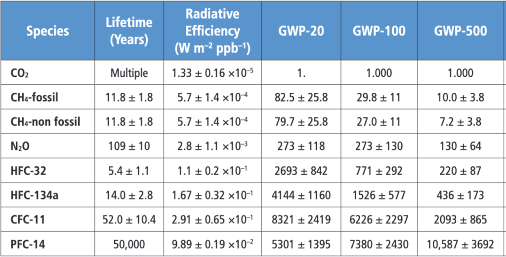
Next take a look at columns four, five, and six. The number at the far end of the hyphen indicates the number of years. We’ll get into it more shortly but, in brief, the gases have different values over different time periods because they have different atmospheric lifetimes. There is nothing special about 20, 100, or 500 years—those are just some numbers the originators of this metric chose to show how it would change over time. Unless otherwise specified, most conversions rely on GWP-100. (I will post more about the surprising history of this metric and the choice of time period here elsewhere.)

See how the GWP values for CO₂ are all 1? That’s because CO₂ is the reference gas, a sort of common currency among greenhouse gases. By setting the table up this way, it makes it very easy to do conversions. For example, if an oil well leaks 1 tonne of CH₄ into the atmosphere, we could use the GWP-100 value to calculate that it released the equivalent of 29.8 tonnes of CO₂ or 29.8 GtCO₂e (It is sometimes also written GtCO₂eq, you can read more on all the different common climate units here.)

The thing is that, although a table in which GWP values are all calculated relative to CO₂ does make it easier to do the most common conversions, it also makes it harder to grasp the underlying concept. For this latter purpose, it will be easier to think in terms of absolute GWP, which I will abbreviate as AGWP to distinguish it from the GWP values in the table above.

In short, AGWP is the time-integrated radiative forcing caused by a greenhouse gas. What does that mean? Take a look at the interactive graphic below.

First get rid of N₂O by typing ‘0’ in the box and hitting return or by moving the slider all the way to the left. Next adjust the other values so that there is 1 GtCO₂ and 1 GtCH₄. Set the years to 0. Year 0 represents the day that the slug of gas was released and the 364 days that followed. (If that seems confusing, think of the way we commonly respond when someone asks us how old we are.)

• GtCO₂: 1
• GtCH₄: 1
• GtN₂O: 0
• Years: 0

Now, in the top chart, titled ‘Slug Emission Radiative Forcing vs Time,’ hover your cursor over each bar. Over the course of year 0 (which is the year that the gas was emitted), you can see that the additional CO₂ in the atmosphere will cause a shift in the earth energy balance of 0.0018 Watts per meter squared. The additional CH4 will cause a shift of about 0.21 Watts per meter squared. Notice that the bottom chart, titled ‘Slug Emission Cumulative Radiative Forcing,’ has the same values as the top chart for now.

Next increase the number of years to 1. Now you can see the radiative forcing caused by the different gasses over two different years. In the top graph, the X axis represents time, so each year is separated. The bottom bar graph is cumulative. Each bar represents the cumulative radiative forcing caused by the gasses over all the years since they were emitted. In other words, imagine taking each of the CH₄ bars from the top graph and stacking them on top of each other to create the CH₄ bar at the bottom. The same goes for CO₂. (Note that the scale of the Y axis is different for the two graphs and will both continue to change each time you adjust one of the inputs.)

Now try setting the years to 100. Look at the cumulative radiative forcing caused by CH₄ and CO₂ in the bottom graph. These values are the absolute GWP for 100 years (AGWP-100), for each gas. The units are in Watts per square meter.

Recall the GWP values from the IPCC table 7.15 that we started with. All GWP values were unitless, and relative to CO₂. To derive them, all we need to do is divide by the AGWP-100 of CO₂. If you divide the AGWP-100 of CO₂ by itself, you will get 1, just as in the table. In other words, if you release 1 gigatonne of CO₂, it is the same as releasing 1 gigatonne of CO₂. Next divide the AGWP-100 of CH₄ by the AGWP-100 of CO₂. Although rounding errors and slightly different parameters may throw it off a little, the value should be close to 29.8, just as in the IPCC table.

Here’s another way of looking at it: if the GWP-100 of CH₄ is 29.8 then, if we release 1 GtCH₄, the cumulative radiative forcing after 100 years should be the same as if we had released 29.8 GtCO₂. To test this, try leaving the CH₄ at 1 gigatonne, and bump the CO₂ up to 29.8 gigatonnes. The bars in the bottom graph should be about the same height, indicating they caused the same amount of cumulative radiative forcing.

Keep playing with the input values. Test out N₂O. Try deriving the GWP-20 and GWP-500 values for CH₄. Try calculating other GWP values, like GWP-1. Note how the GWP values change over different time periods as a result of the different lifetimes of the different gasses.

Once you are feeling comfortable, set the values to 29.8 GtCO₂ and 1 GtCH₄ over 100 years. Look at the bottom graph. The cumulative radiative forcing bars for each gas should be about the same height. When someone says that 1 GtCH₄ is equivalent to 29.8 GtCO₂, that’s what they are talking about. Now look at the top graph on the top, though. See the problem? Methane has a huge impact in the first few years, and almost none after about 40 or 50 years. In any given year following an emission, the effects of different gases will not the same at all! GWP is such a deeply flawed metric with such huge policy ramifications that even the scientists who first came up with it were aghast, a topic I will cover in a future post.